Robust Scene Text Recognition with Automatic Rectification

Robust Scene Text Recognition with Automatic Rectiﬁcation

Baoguang Shi, Xinggang Wang, Pengyuan Lyu, Cong Yao, Xiang Bai

∗

School of Electronic Information and Communications

Huazhong University of Science and Technology

[email protected], [email protected]

Abstract

Recognizing text in natural images is a challenging task

with many unsolved problems. Different from those in

documents, words in natural images often possess irreg-

ular shapes, which are caused by perspective distortion,

curved character placement, etc. We propose RARE (Robust

text recognizer with Automatic REctiﬁcation), a recognition

model that is robust to irregular text. RARE is a specially-

designed deep neural network, which consists of a Spatial

Transformer Network (STN) and a Sequence Recognition

Network (SRN). In testing, an image is ﬁrstly rectiﬁed via

a predicted Thin-Plate-Spline (TPS) transformation, into a

more “readable” image for the following SRN, which rec-

ognizes text through a sequence recognition approach. We

show that the model is able to recognize several types of

irregular text, including perspective text and curved text.

RARE is end-to-end trainable, requiring only images and

associated text labels, making it convenient to train and

deploy the model in practical systems. State-of-the-art or

highly-competitive performance achieved on several bench-

marks well demonstrates the effectiveness of the proposed

model.

1. Introduction

In natural scenes, text appears on various kinds of ob-

jects, e.g. road signs, billboards, and product packaging. It

carries rich and high-level semantic information that is im-

portant for image understanding. Recognizing text in im-

ages facilitates many real-world applications, such as geo-

location, driverless car, and image-based machine transla-

tion. For these reasons, scene text recognition has attracted

great interest from the community [28, 37, 15]. Despite the

maturity of the research on Optical Character Recognition

(OCR) [26], recognizing text in natural images, rather than

scanned documents, is still challenging. Scene text images

exhibit large variations in the aspects of illumination, mo-

∗

Corresponding author

Spatial

Transformer

Network

Sequence

Recognition

Network

Rectiﬁed ImageInput Image

"MOON"

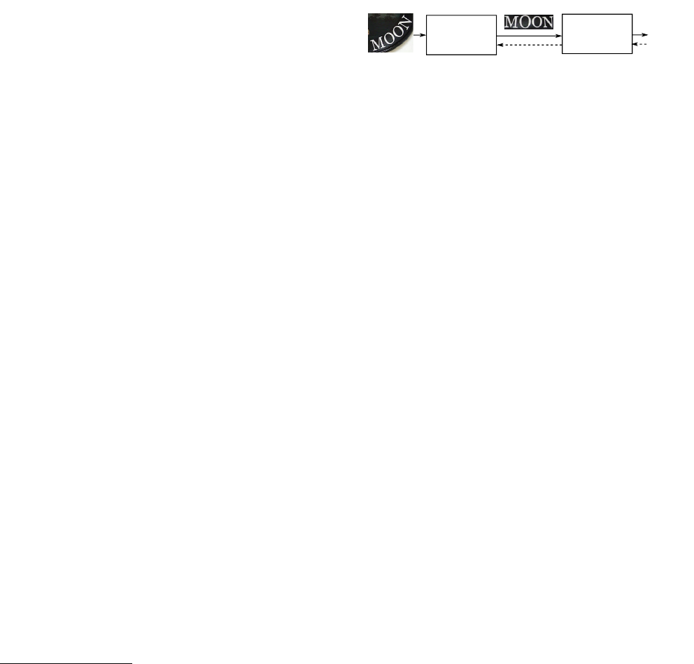
Figure 1. Schematic overview of RARE, which consists a spatial

transformer network (STN) and a sequence recognition network

(SRN). The STN transforms an input image to a rectiﬁed im-

age, while the SRN recognizes text. The two networks are jointly

trained by the back-propagation algorithm [22]. The dashed lines

represent the ﬂows of the back-propagated gradients.

tion blur, text font, color, etc. Moreover, text in the wild

may have irregular shape. For example, some scene text is

perspective text [29], which is caused by side-view camera

angles; some has curved shapes, meaning that its characters

are placed along curves rather than straight lines. We call

such text irregular text, in contrast to regular text which is

horizontal and frontal.

Usually, a text recognizer works best when its input im-

ages contain tightly-bounded regular text. This motivates

us to apply a spatial transformation prior to recognition, in

order to rectify input images into ones that are more “read-

able” by recognizers. In this paper, we propose a recog-

nition method that is robust to irregular text. Speciﬁcally,

we construct a deep neural network that combines a Spatial

Transformer Network [18] (STN) and a Sequence Recogni-

tion Network (SRN). An overview of the model is given in

Fig. 1.

In the STN, an input image is spatially transformed into

a rectiﬁed image. Ideally, the STN produces an image that

contains regular text, which is a more appropriate input for

the SRN than the original one. The transformation is a thin-

plate-spline [6] (TPS) transformation, whose nonlinearity

allows us to rectify various types of irregular text, includ-

ing perspective and curved text. The TPS transformation is

conﬁgured by a set of ﬁducial points, whose coordinates are

regressed by a convolutional neural network.

In an image that contains regular text, characters are ar-

ranged along a horizontal line. It bares some resemblance

arXiv:1603.03915v2 [cs.CV] 19 Apr 2016

to a sequential signal. Motivated by this, for the SRN we

construct an attention-based model [4] that recognizes text

in a sequence recognition approach. The SRN consists of

an encoder and a decoder. Given an input image, the en-

coder generates a sequential feature representation, which

is a sequence of feature vectors. The decoder recurrently

generates a character sequence conditioning on the input

sequence, by decoding the relevant contents which are de-

termined by its attention mechanism at each step.

We show that, with proper initialization, the whole

model can be trained end-to-end. Consequently, for the

STN, we do not need to label any geometric ground truth,

i.e. the positions of the TPS ﬁducial points, but let its train-

ing be supervised by the error differentials back-propagated

by the SRN. In practice, the training eventually makes the

STN tend to produce images that contain regular text, which

are desirable inputs for the SRN.

The contributions of this paper are three-fold: First, we

propose a novel scene text recognition method that is ro-

bust to irregular text. Second, our model extends the STN

framework [18] with an attention-based model. The original

STN is only tested on plain convolutional neural networks.

Third, our model adopts a convolutional-recurrent structure

in the encoder of the SRN, thus is a novel variant of the

attention-based model [4].

2. Related Work

In recent years, a rich body of literature concerning

scene text recognition has been published. Comprehensive

surveys have been given in [40, 44]. Among the tradi-

tional methods, many adopt bottom-up approaches, where

individual characters are ﬁrstly detected using sliding win-

dow [36, 35], connected components [28], or Hough vot-

ing [39]. Following that, the detected characters are in-

tegrated into words by means of dynamic programming,

lexicon search [35], etc.. Other work adopts top-down ap-

proaches, where text is directly recognized from entire in-

put images, rather than detecting and recognizing individual

characters. For example, Alm

azan et al. [2] propose to pre-

dict label embedding vectors from input images. Jaderberg

et al. [17] address text recognition with a 90k-class con-

volutional neural network, where each class corresponds to

an English word. In [16], a CNN with a structured out-

put layer is constructed for unconstrained text recognition.

Some recent work models the problem as a sequence recog-

nition problem, where text is represented by character se-

quence. Su and Lu [34] extract sequential image represen-

tation, which is a sequence of HOG [10] descriptors, and

predict the corresponding character sequence with a recur-

rent neural network (RNN). Shi et al. [32] propose an end-

to-end sequence recognition network which combines CNN

and RNN. Our method also adopts the sequence prediction

scheme, but we further take the problem of irregular text

into account.

Although being common in the tasks of scene text de-

tection and recognition, the issue of irregular text is rela-

tively less addressed in explicit ways. Yao et al. [38] ﬁrstly

propose the multi-oriented text detection problem, and deal

with it by carefully designing rotation-invariant region de-

scriptors. Zhang et al. [42] propose a character rectiﬁcation

method that leverages the low-rank structures of text. Phan

et al. propose to explicitly rectify perspective distortions via

SIFT [23] descriptor matching. The above-mentioned work

brings insightful ideas into this issue. However, most meth-

ods deal with only one type of irregular text with speciﬁ-

cally designed schemes. Our method rectiﬁes several types

of irregular text in a uniﬁed way. Moreover, it does not re-

quire extra annotations for the rectiﬁcation process, since

the STN is supervised by the SRN during training.

3. Proposed Model

In this section we formulate our model. Overall, the

model takes an input image I and outputs a sequence l =

, . . . , l

), where l

is the t-th character, T is the variable

string length.

3.1. Spatial Transformer Network

The STN transforms an input image I to a rectiﬁed im-

age I

with a predicted TPS transformation. It follows the

framework proposed in [18]. As illustrated in Fig. 2, it ﬁrst

predicts a set of ﬁducial points via its localization network.

Then, inside the grid generator, it calculates the TPS trans-

formation parameters from the ﬁducial points, and gener-

ates a sampling grid on I. The sampler takes both the grid

and the input image, it produces a rectiﬁed image I

by sam-

pling on the grid points.

A distinctive property of STN is that its sampler is dif-

ferentiable. Therefore, once we have a differentiable local-

ization network and a differentiable grid generator, the STN

can back-propagate error differentials and gets trained.

Input Image

Fiducial Points

Loalization

Network

Sampler V

Grid

Generator

Rectiﬁed Image

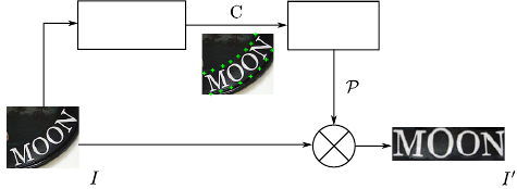
Figure 2. Structure of the STN. The localization network localizes

a set of ﬁducial points C, with which the grid generator generates

a sampling grid P. The sampler produces a rectiﬁed image I

given I and P .

3.1.1 Localization Network

The localization network localizes K ﬁducial points by di-

rectly regressing their x, y-coordinates. Here, constant K

is an even number. The coordinates are denoted by C =

, . . . , c

] ∈ <

2×K

, whose k-th column c

= [x

, y

]

contains the coordinates of the k-th ﬁducial point. We use

a normalized coordinate system whose origin is the image

center, so that x

, y

are within the range of [−1, 1].

We use a convolutional neural network (CNN) for the

regression. Similar to the conventional structures [33, 21],

the CNN contains convolutional layers, pooling layers and

fully-connected layers. However, we use it for regression

instead of classiﬁcation. For the output layer, which is

the last fully-connected layer, we set the number of output

nodes to 2K and the activation function to tanh(·), so that

its output vectors have values that are within the range of

(−1, 1). Last, the output vector is reshaped into C.

The network localizes ﬁducial points based on global im-

age contexts. It is expected to capture the overall text shape

of an input image, and localizes ﬁducial points accordingly.

It should be emphasized that we do not annotate coordinates

of ﬁducial points for any sample. Instead, the training of the

localization network is completely supervised by the gradi-

ents propagated by the other parts of the STN, following the

back-propagation algorithm [22].

3.1.2 Grid Generator

The grid generator estimates the TPS transformation param-

eters, and generates a sampling grid. We ﬁrst deﬁne another

set of ﬁducial points, called the base ﬁducial points, de-

noted by C

= [c

, . . . , c

] ∈ <

2×K

. As illustrated in

Fig. 3, the base ﬁducial points are evenly distributed along

the top and bottom edge of a rectiﬁed image I

. Since K

is a constant and the coordinate system is normalized, C

always a constant.

Input Image

Rectiﬁed Image

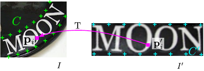
Figure 3. Fiducial points and the TPS transformation. Green mark-

ers on the left image are the ﬁducial points C. Cyan markers on

the right image are the base ﬁducial points C

. The transformation

T is represented by the pink arrow. For a point (x

, y

) on I

, the

transformation T ﬁnds the corresponding point (x

, y

) on I.

The parameters of the TPS transformation is represented

by a matrix T ∈ <

2×(K+3)

, which is computed by

T =



∆

−1



3×2



, (1)

where ∆

∈ <

(K+3)×(K+3)

is a matrix determined only

by C

, thus also a constant:

∆





K×1

0 0 1

1×K

0 0 C





where the element on the i-th row and j-th column of R is

i,j

= d

i,j

ln d

i,j

, d

i,j

is the euclidean distance between c

and c

The grid of pixels on a rectiﬁed image I

is denoted

by P

= {p

}

i=1,...,N

, where p

= [x

, y

]

is the x,y-

coordinates of the i-th pixel, N is the number of pixels. As

illustrated in Fig. 3, for every point p

on I

, we ﬁnd the

corresponding point p

= [x

, y

]

on I, by applying the

transformation:

i,k

= d

i,k

ln d

i,k

(2)



1, x

, y

, r

i,1

, . . . , r

i,K



(3)

= T

, (4)

where d

i,k

is the euclidean distance between p

and the k-th

base ﬁducial point c

By iterating over all points in P

, we generate a grid

P = {p

}

i=1,...,N

on the input image I. The grid generator

can back-propagate gradients, since its two matrix multipli-

cations, Eq. 1 and Eq. 4, are both differentiable.

3.1.3 Sampler

Lastly, in the sampler, the pixel value of p

is bilinearly

interpolated from the pixels near p

on the input image. By

setting all pixel values, we get the rectiﬁed image I

= V (P, I), (5)

where V represents the bilinear sampler [18], which is also

a differentiable module.

The ﬂexibility of the TPS transformation allows us to

transform irregular text images into rectiﬁed images that

contain regular text. In Fig. 4, we show some common types

of irregular text, including a) loosely-bounded text, which

resulted by imperfect text detection; b) multi-oriented text,

caused by non-horizontal camera views; c) perspective text,

caused by side-view camera angles; d) curved text, a com-

monly seen artistic style. The STN is able to rectify images

that contain these types of irregular text, making them more

readable for the following recognizer.

3.2. Sequence Recognition Network

Since target words are inherently sequences of charac-

ters, we model the recognition problem as a sequence recog-

nition problem, and address it with a sequence recognition

network. The input to the SRN is a rectiﬁed image I

, which

Input Image Rectiﬁed Image

(a)

(b)

(c)

(d)

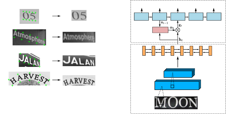
Figure 4. The STN rectiﬁes images that contain several types of

irregular text. Green markers are the predicted ﬁducial points on

the input images. The STN can deal with several types of irregular

text, including (a) loosely-bounded text; (b) multi-oriented text;

ideally contains a word that is written horizontally from left

to right. We extract a sequential representation from I

, and

recognize a word from it.

In our model, the SRN is an attention-based model [4, 8],

which directly recognizes a sequence from an input image.

The SRN consists of an encoder and a decoder. The encoder

extracts a sequential representation from the input image I

The decoder recurrently generates a sequence conditioned

on the sequential representation, by decoding the relevant

contents it attends to at each step.

3.2.1 Encoder: Convolutional-Recurrent Network

A na

ıve approach for extracting a sequential representation

for I

is to take local image patches from left to right, and

describe each of them with a CNN. However, this approach

does not share the computation among overlapping patches,

thus inefﬁcient. Besides, the spatial dependencies between

the patches are not exploited and leveraged. Instead, follow-

ing [32], we build a network that combines convolutional

layers and recurrent networks. The network extracts a se-

quence of feature vectors, given an input image of arbitrary

size.

As illustrated in Fig. 5, at the bottom of the encoder is

several convolutional layers. They produce feature maps

that are robust and high-level descriptions of an input im-

age. Suppose the feature maps have the size D

conv

× W

conv

, where D

conv

is the depth, and H

conv

are the height and width respectively. The next oper-

ation is to convert the maps into a sequence of W

conv

vec-

tors, each has D

conv

dimensions. Speciﬁcally, the

“map-to-sequence” operation takes out the columns of the

GRU

Map-to-sequence

Decoder

Encoder

BLSTM

ConvNet

Input image

GRU GRU GRU GRU

<EOS>'N''O''O'

'M'

Attend

Figure 5. Structure of the SRN, which consists of an encoder and

a decoder. The encoder uses several convolution layers (ConvNet)

and a two-layer BLSTM network to extract a sequential represen-

tation (h) for the input image. The decoder generates a character

sequence (including the EOS token) conditioned on h.

maps in the left-to-right order, and ﬂattens them into vec-

tors. According to the translation invariance property of

CNN, each vector corresponds to a local image region, i.e.

receptive ﬁeld, and is a descriptor for that region.

Restricted by the sizes of the receptive ﬁelds, the fea-

ture sequence leverages limited image contexts. We further

apply a two-layer Bidirectional Long-Short Term Mem-

ory (BLSTM) [14, 13] network to the sequence, in order

to model the long-term dependencies within the sequence.

The BLSTM is a recurrent network that can analyze the de-

pendencies within a sequence in both directions, it outputs

another sequence which has the same length as the input

one. The output sequence is h = (h

, . . . , h

), where

L = W

conv

3.2.2 Decoder: Recurrent Character Generator

The decoder recurrently generates a sequence of characters,

conditioned on the sequence produced by the encoder. It is

a recurrent neural network with the attention structure pro-

posed in [4, 8]. In the recurrency part, we adopt the Gated

Recurrent Unit (GRU) [7] as the cell.

The generation is a T -step process, at step t, the decoder

computes a vector of attention weights α

∈ <

via the

attention process described in [8]:

= Attend(s

t−1

, α

t−1

, h), (6)

where s

t−1

is the state variable of the GRU cell at the last

step. For t = 1, both s

and α

are zero vectors. Then, a

glimpse g

is computed by linearly combining the vectors

in h: g

i=1

. Since α

has non-negative values

that sum to one, it effectively controls where the decoder

focuses on.

The state s

t−1

is updated via the recurrent process of

GRU [7, 8]:

= GRU(l

t−1

, g

, s

t−1

), (7)

where l

t−1

is the (t − 1)-th ground-truth label in training,

while in testing, it is the label predicted in the previous step,

i.e.

t−1

The probability distribution over the label space is esti-

mated by:

= softmax(W

). (8)

Following that, a character

is predicted by taking the class

with the highest probability. The label space includes all

English alphanumeric characters, plus a special “end-of-

sequence” (EOS) token, which ends the generation process.

The SRN directly maps a input sequence to another se-

quence. Both input and output sequences may have arbi-

trary lengths. It can be trained with only word images and

associated text.

3.3. Model Training

We denote the training set by X = {(I

(i)

, l

(i)

)}

i=1...N

To train the model, we minimize the negative log-likelihood

over X :

L =

i=1

log

(i)

t=1

p(l

(i)

; θ), (9)

where the probability p(·) is computed by Eq. 8, θ is the pa-

rameters of both STN and SRN. The optimization algorithm

is the ADADELTA [41], which we ﬁnd fast in convergence

speed.

(a) (b) (c)

Figure 6. Some initialization patterns for the ﬁducial points.

The model parameters are randomly initialized, except

the localization network, whose output fully-connected

layer is initialized by setting weights to zero. The initial

biases are set to such values that yield the ﬁducial points

pattern displayed in Fig. 6.a. Empirically, we also ﬁnd that

the patterns displayed Fig. 6.b and Fig. 6.c yield relatively

poorer performance. Randomly initializing the localization

network results in failure of convergence during training.

0.2

0.6

0.8

0.1

Figure 7. A preﬁx tree of three words: “ten”, “tea”, and “to”.  and

Ω are the tree root and the EOS token respectively. The recognition

starts from the tree root. At each step the posterior probabilities of

all child nodes are computed. The child node with the highest

probability is selected as the next node. The process iterates until

a leaf node is reached. Numbers on the edges are the posterior

probabilities. Blue nodes are the selected nodes. In this case, the

predicted word is “tea”.

3.4. Recognizing With a Lexicon

When a test image is associated with a lexicon, i.e. a set

of words for selection, the recognition process is to pick the

word with the highest posterior conditional probability:

∗

= arg max

log

|l|

t=1

p(l

|I; θ). (10)

However, on very large lexicons, e.g. the Hunspell [1]

which contains more than 50k words, computing Eq. 10

is time consuming, as it requires iterating over all lexicon

words. We adopt an efﬁcient approximate search scheme

on large lexicons. The motivation is that computation can

be shared among words that share the same preﬁx.

We ﬁrst construct a preﬁx tree over a given lexicon. As

illustrated in Fig. 7, each node of the tree is a character la-

bel. Nodes on a path from the root to a leaf forms a word

(including the EOS). In testing, we start from the root node,

every time the model outputs a distribution

, the child

node with the highest posterior probability is selected as the

next node to move to. The process repeats until a leaf node

is reached, and a word is found on the path from the root to

that leaf. Since the tree depth is at most the length of the

longest word in the lexicon, this search process takes much

less computation than the precise search.

Recognition performance could be further improved by

incorporating beam search. A list of nodes is maintained,

and the above search process is repeated on each of them.

After each step, the list is updated to store the nodes with

top-B accumulated log-likelihoods, where B is the beam

width. Larger beam width usually results in better perfor-

mance, but lower search speed.

Table 1. Recognition accuracies on general recognition benchmarks. The titles “50”, “1k” and “50k” are lexicon sizes. The “Full” lexicon

contains all per-image lexicon words. “None” means recognition without a lexicon.

Method

IIIT5K SVT IC03 IC13

50 1k None 50 None 50 Full 50k None None

ABBYY [35] 24.3 - - 35.0 - 56.0 55.0 - - -

Wang et al. [35] - - - 57.0 - 76.0 62.0 - - -

Mishra et al. [25] 64.1 57.5 - 73.2 - 81.8 67.8 - - -

Wang et al. [37] - - - 70.0 - 90.0 84.0 - - -

Goel et al. [11] - - - 77.3 - 89.7 - - - -

Bissacco et al. [5] - - - 90.4 78.0 - - - - 87.6

Alsharif and Pineau [3] - - - 74.3 - 93.1 88.6 85.1 - -

Almaz

an et al. [2] 91.2 82.1 - 89.2 - - - - - -

Yao et al. [39] 80.2 69.3 - 75.9 - 88.5 80.3 - - -

Rodrguez-Serrano et al. [31] 76.1 57.4 - 70.0 - - - - - -

Jaderberg et al. [19] - - - 86.1 - 96.2 91.5 - - -

Su and Lu [34] - - - 83.0 - 92.0 82.0 - - -

Gordo [12] 93.3 86.6 - 91.8 - - - - - -

Jaderberg et al. [17] 97.1 92.7 - 95.4 80.7 98.7 98.6 93.3 93.1 90.8

Jaderberg et al. [16] 95.5 89.6 - 93.2 71.7 97.8 97.0 93.4 89.6 81.8

Shi et al. [32] 97.6 94.4 78.2 96.4 80.8 98.7 97.6 95.5 89.4 86.7

RARE 96.2 93.8 81.9 95.5 81.9 98.3 96.2 94.8 90.1 88.6

RARE (SRN only) 96.5 92.8 79.7 96.1 81.5 97.8 96.4 93.7 88.7 87.5

4. Experiments

In this section we evaluate our model on a number of

standard scene text recognition benchmarks, paying special

attention to recognition performance on irregular text. First

we evaluate our model on some general recognition bench-

marks, which mainly consist of regular text, but irregular

text also exists. Next, we perform evaluations on bench-

marks that are specially designed for irregular text recogni-

tion. For all benchmarks, performance is measured by word

accuracy.

4.1. Implementation Details

Spatial Transformer Network The localization network

of STN has 4 convolution layers, each followed by a 2 × 2

max-pooling layer. The ﬁlter size, padding size and stride

are 3, 1, 1 respectively, for all convolutional layers. The

number of ﬁlters are respectively 64, 128, 256 and 512. Fol-

lowing the convolutional and the max-pooling layers is two

fully-connected layers with 1024 hidden units. We set the

number of ﬁducial points to K = 20, meaning that the lo-

calization network outputs a 40-dimensional vector. Acti-

vation functions for all layers are the ReLU [27], except the

output layer which uses tanh(·).

Sequence Recognition Network In the SRN, the en-

coder has 7 convolutional layers, whose {ﬁlter size,

number of ﬁlters, stride, padding size} are respec-

tively {3,64,1,1}, {3,128,1,1}, {3,256,1,1}, {3,256,1,1,},

{3,512,1,1}, {3,512,1,1}, and {2,512,1,0}. The 1st, 2nd,

4th, 6th convolutional layers are each followed by a 2 × 2

max-pooling layer. On the top of the convolutional layers

is a two-layer BLSTM network, each LSTM has 256 hid-

den units. For the decoder, we use a GRU cell that has 256

memory blocks and 37 output units (26 letters, 10 digits,

and 1 EOS token).

Model Training Our model is trained on the 8-million

synthetic samples released by Jaderberg et al. [15]. No extra

data is used. The batch size is set to 64 in training. Follow-

ing [17, 16], images are resized to 100 × 32 in both training

and testing. The output size of the STN is also 100×32. Our

model processes ∼160 samples per second during training,

and converges in 2 days after ∼3 epochs over the training

dataset.

Implementation We implement our model under the

Torch7 framework [9]. Most parts of the model are GPU-

accelerated. All our experiments are carried out on a work-

station which has one Intel Xeon(R) E5-2620 2.40GHz

CPU, an NVIDIA GTX-Titan GPU, and 64GB RAM.

Without a lexicon, the model takes less than 2ms recog-

nizing an image. With a lexicon, recognition speed depends

on the lexicon size. We adopt the precise search (Sec. 3.4)

when lexicon size ≤ 1k. On larger lexicons, we adopt the

approximate beam search (Sec. 3.4) with a beam width of

7. With a 50k-word lexicon, the search takes ∼200ms per

image.

4.2. Results on General Benchmarks

Our model is ﬁrstly evaluated on benchmarks that are de-

signed for general scene text recognition tasks. Samples in

these benchmarks mostly contain regular text, but irregular

text also exists. The benchmark datasets are:

• IIIT 5K-Words [25] (IIIT5K) contains 3000 cropped

word images for testing. The images are collected

from the Internet. For each image, there is a 50-word

lexicon and a 1000-word lexicon. All lexicons con-

sist of a ground truth word and some randomly picked

words.

• Street View Text [35] (SVT) is collected from Google

Street View. Its test dataset consists of 647 word im-

ages. Many images in SVT are severely corrupted by

noise and blur, or have very low resolutions. Each sam-

ple is associated with a 50-word lexicon.

• ICDAR 2003 [24] (IC03) contains 860 cropped word

images, each associated with a 50-word lexicon de-

ﬁned by Wang et al. [35]. Following [35], we dis-

card images that contain non-alphanumeric characters

or have less than three characters. Besides, there is a

“full lexicon” which contains all lexicon words, and

the Hunspell [1] lexicon which has 50k words.

• ICDAR 2013 [20] (IC13) inherits most of its samples

from IC03. After ﬁltering samples as done in IC03, the

dataset contains 857 samples.

In Tab. 1 we report our results, and compare them with

other methods. On unconstrained recognition tasks (rec-

ognizing without a lexicon), our model outperforms all the

other methods in comparison. On IIIT5K, RARE outper-

forms prior art CRNN [32] by nearly 4 percentages, indi-

cating a clear improvement in performance. We observe

that IIIT5K contains a lot of irregular text, especially curved

text, while RARE has an advantage in dealing with irregu-

lar text. Note that, although our model falls behind [17] on

some datasets, our model differs from [17] in that it is able

recognize random strings such as telephone numbers, while

[17] only recognizes words that are in its 90k-dictionary.

On constrained recognition tasks (recognizing with a lexi-

con), RARE achieves state-of-the-art or highly competitive

accuracies. On IIIT5K, SVT and IC03, constrained recog-

nition accuracies are on par with [17], and slightly lower

than [32].

We also train and test a model that contains only the

SRN. As reported in the last row of Tab. 1, we see that

the SRN-only model is also a very competitive recognizer,

achieving higher or competitive performance on most of the

benchmarks.

4.3. Recognizing Perspective Text

To validate the effectiveness of the rectiﬁcation scheme,

we evaluate RARE on the task of perspective text recog-

nition. SVT-Perspective [29] is speciﬁcally designed for

evaluating performance of perspective text recognition al-

gorithms. Text samples in SVT-Perspective are picked from

side view angles in Google Street View, thus most of them

are heavily deformed by perspective distortion. Some ex-

amples are shown in Fig. 8.a. SVT-Perspective consists

of 639 cropped images for testing. Each image is associ-

ated with a 50-word lexicon, which is inherited from the

SVT [35] dataset. In addition, there is a “Full” lexicon

which contains all the per-image lexicon words.

(a)

(b)

Figure 8. Examples of irregular text. a) Perspective text. Samples

are taken from the SVT-Perspective [29] dataset; b) Curved text.

Samples are taken from the CUTE80 [30] dataset.

We use the same model trained on the synthetic dataset

without ﬁne-tuning. For comparison, we test the CRNN

model [32] on SVT-Perspective. We also compare RARE

with [35, 25, 37, 29], whose recognition accuracies are re-

ported in [29].

Table 2. Recognition accuracies on SVT-Perspective [29]. “50”

and “Full” represent recognition with 50-word lexicons and the

full lexicon respectively. “None” represents recognition without a

lexicon.

Method 50 Full None

Wang et al. [35] 40.5 26.1 -

Mishra et al. [25] 45.7 24.7 -

Wang et al. [37] 40.2 32.4 -

Phan et al. [29] 75.6 67.0 -

Shi et al. [32] 92.6 72.6 66.8

RARE 91.2 77.4 71.8

Tab. 2 summarizes the results. In the second and third

columns, we compare the accuracies of recognition with the

50-word lexicon and the full lexicon. Our method outper-

forms [29], which is a perspective text recognition method,

by a large margin on both lexicons. However, this gap

is partially due to that we use a much larger training set

than [29]. In the comparisons with [32], which uses the

same training set as RARE, we still observe signiﬁcant im-

provements in both the Full lexicon and the lexicon-free

settings. Furthermore, recall the results in Tab. 1, on SVT-

Perspective RARE outperforms [32] by a even larger mar-

gin. The reason is that the SVT-perspective dataset mainly

consists of perspective text, which is inappropriate for di-

rect recognition. Our rectiﬁcation scheme can signiﬁcantly

alleviate this problem.

In Fig. 9 we present some qualitative analysis. Fiducial

points predicted by the STN are plotted on input images in

green crosses. We see that the STN tends to place ﬁdu-

cial points along upper and lower edges of scene text, and

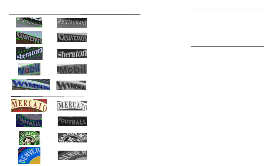
restaurant

quiznos

sheraton

mobil

Pred

Input Image Rectified Image

mercato

marcato

football

staming

starbucks

stinker

denver

SVT-Perspective

CUTE80

windwin

wyndham

Figure 9. Examples showing the rectiﬁcations our model makes

and the recognition results. The left column is the input images,

where green crosses are the predicted ﬁducial points. The mid-

dle column is the rectiﬁed images (we use gray-scale images for

recognition). The right column is the recognized text and the

ground truth text. Green and red characters are correctly and mis-

takenly recognized characters, respectively. The ﬁrst ﬁve rows

are taken from SVT-Perspective [29], the rest rows are taken from

CUTE80 [30].

hence produces rectiﬁed images that are more readable for

the SRN. However, the STN fails sometimes in the case of

heavy perspective distortion.

4.4. Recognizing Curved Text

Curved text is a commonly seen artistic-style text in nat-

ural scenes. Due to its irregular character placement, rec-

ognizing curved text is very challenging. CUTE80 [30] fo-

cuses on the recognition of curved text. The dataset contains

80 high-resolution images taken in natural scenes. Origi-

nally, the dataset is proposed for detection tasks. We crop

the words, resulting in 288 word images for testing. For

comparisons, we evaluate the trained models of [17] and

[32]. All models are evaluated without a lexicon.

From the results summarized in Tab. 3, we see that

RARE outperforms the other two methods by a large mar-

gin. [17] is a constrained recognition model, it cannot rec-

ognize words that are not in its dictionary. [32] is able to

recognize arbitrary words, but it does not have a speciﬁc

mechanism for handling curved text. Our model rectiﬁes

Table 3. Recognition accuracies on CUTE80 [29].

Method Accuracy

Jaderberg et al. [17] 42.7

Shi et al. [32] 54.9

RARE 59.2

images that contain curved text before recognizing them.

Therefore, it is advantageous on this task.

In Fig. 9, we demonstrate the effect of rectiﬁcation

through some examples. Generally, the rectiﬁcation made

by the STN is not perfect, but it alleviates the recognition

difﬁculty to some extent. RARE tends to fail when curve

angles are too large, as shown in the last two rows of Fig. 9.

5. Conclusion

We study a common but difﬁcult problem in scene text

recognition, called the irregular text problem. Traditional

solutions typically use a separate text rectiﬁcation compo-

nent. We address this problem in a more feasible and el-

egant way by adopting a differentiable spatial transformer

network module. In addition, the spatial transformer net-

work is connected to an attention-based sequence recog-

nizer, allowing us to train the whole model end-to-end. The

extensive experimental results show that 1) without geomet-

ric supervision, the learned model can automatically gen-

erate more “readable” images for both human and the se-

quence recognition network; 2) the proposed text rectiﬁ-

cation method can signiﬁcantly improve recognition accu-

racies on irregular scene text; 3) the proposed scene text

recognition system is competitive compared with the state-

of-the-arts. In the future, we plan to address the end-to-

end scene text reading problem through the combination of

RARE with a scene text detection method, e.g. [43].

Acknowledgments

This work was primarily supported by National Natural

Science Foundation of China (NSFC) (No. 61222308, No.

61573160 and No. 61503145), and Open Project Program

of the State Key Laboratory of Digital Publishing Technol-

ogy (No. F2016001).

References

[1] Hunspell. http://hunspell.sourceforge.net/.

[2] J. Almaz

an, A. Gordo, A. Forn

es, and E. Valveny. Word spot-

ting and recognition with embedded attributes. IEEE Trans.

Pattern Anal. Mach. Intell., 36(12):2552–2566, 2014.

[3] O. Alsharif and J. Pineau. End-to-end text recognition with

hybrid hmm maxout models. ICLR, 2014.

[4] D. Bahdanau, K. Cho, and Y. Bengio. Neural machine

translation by jointly learning to align and translate. CoRR,

abs/1409.0473, 2014.

[5] A. Bissacco, M. Cummins, Y. Netzer, and H. Neven. Pho-

toocr: Reading text in uncontrolled conditions. In ICCV,

2013.

[6] F. L. Bookstein. Principal warps: Thin-plate splines and the

decomposition of deformations. IEEE Trans. Pattern Anal.

Mach. Intell., 11(6):567–585, 1989.

[7] K. Cho, B. van Merrienboer, D. Bahdanau, and Y. Bengio.

On the properties of neural machine translation: Encoder-

decoder approaches. CoRR, abs/1409.1259, 2014.

[8] J. Chorowski, D. Bahdanau, D. Serdyuk, K. Cho, and Y. Ben-

gio. Attention-based models for speech recognition. CoRR,

abs/1506.07503, 2015.

[9] R. Collobert, K. Kavukcuoglu, and C. Farabet. Torch7: A

matlab-like environment for machine learning. In BigLearn,

NIPS Workshop, 2011.

[10] N. Dalal and B. Triggs. Histograms of oriented gradients for

human detection. In CVPR, 2005.

[11] V. Goel, A. Mishra, K. Alahari, and C. V. Jawahar. Whole is

greater than sum of parts: Recognizing scene text words. In

ICDAR, 2013.

[12] A. Gordo. Supervised mid-level features for word image rep-

resentation. In CVPR, 2015.

[13] A. Graves, A. Mohamed, and G. E. Hinton. Speech recogni-

tion with deep recurrent neural networks. In ICASSP, 2013.

[14] S. Hochreiter and J. Schmidhuber. Long short-term memory.

Neural Computation, 9(8):1735–1780, 1997.

[15] M. Jaderberg, K. Simonyan, A. Vedaldi, and A. Zisserman.

Synthetic data and artiﬁcial neural networks for natural scene

text recognition. NIPS Deep Learning Workshop, 2014.

[16] M. Jaderberg, K. Simonyan, A. Vedaldi, and A. Zisserman.

Deep structured output learning for unconstrained text recog-

nition. In ICLR, 2015.

[17] M. Jaderberg, K. Simonyan, A. Vedaldi, and A. Zisserman.

Reading text in the wild with convolutional neural networks.

Int. J. Comput. Vision, 2015.

[18] M. Jaderberg, K. Simonyan, A. Zisserman, and

K. Kavukcuoglu. Spatial transformer networks. CoRR,

abs/1506.02025, 2015.

[19] M. Jaderberg, A. Vedaldi, and A. Zisserman. Deep features

for text spotting. In ECCV, 2014.

[20] D. Karatzas, F. Shafait, S. Uchida, M. Iwamura, L. G. i Big-

orda, S. R. Mestre, J. Mas, D. F. Mota, J. Almaz

an, and

L. de las Heras. ICDAR 2013 robust reading competition.

In ICDAR, 2013.

[21] A. Krizhevsky, I. Sutskever, and G. E. Hinton. Imagenet

classiﬁcation with deep convolutional neural networks. In

NIPS, 2012.

[22] Y. LeCun, L. Bottou, Y. Bengio, and P. Haffner. Gradient-

based learning applied to document recognition. Proceed-

ings of the IEEE, 86(11):2278–2324, 1998.

[23] D. G. Lowe. Distinctive image features from scale-invariant

keypoints. Int. J. Comput. Vision, 60(2):91–110, 2004.

[24] S. M. Lucas, A. Panaretos, L. Sosa, A. Tang, S. Wong,

R. Young, K. Ashida, H. Nagai, M. Okamoto, H. Yamamoto,

H. Miyao, J. Zhu, W. Ou, C. Wolf, J. Jolion, L. Todoran,

M. Worring, and X. Lin. ICDAR 2003 robust reading com-

petitions: entries, results, and future directions. IJDAR, 7(2-

3):105–122, 2005.

[25] A. Mishra, K. Alahari, and C. V. Jawahar. Scene text recog-

nition using higher order language priors. In BMVC, 2012.

[26] G. Nagy. Twenty years of document image analysis in PAMI.

IEEE Trans. Pattern Anal. Mach. Intell., 22(1):38–62, 2000.

[27] V. Nair and G. E. Hinton. Rectiﬁed linear units improve re-

stricted boltzmann machines. In ICML, 2010.

[28] L. Neumann and J. Matas. Real-time scene text localization

and recognition. In CVPR, 2012.

[29] T. Q. Phan, P. Shivakumara, S. Tian, and C. L. Tan. Recog-

nizing text with perspective distortion in natural scenes. In

ICCV, 2013.

[30] A. Risnumawan, P. Shivakumara, C. S. Chan, and C. L. Tan.

A robust arbitrary text detection system for natural scene im-

ages. Expert Syst. Appl., 41(18):8027–8048, 2014.

[31] J. A. Rodr

ıguez-Serrano, A. Gordo, and F. Perronnin. Label

embedding: A frugal baseline for text recognition. Int. J.

Comput. Vision, 113(3):193–207, 2015.

[32] B. Shi, X. Bai, and C. Yao. An end-to-end trainable neural

network for image-based sequence recognition and its ap-

plication to scene text recognition. CoRR, abs/1507.05717,

2015.

[33] K. Simonyan and A. Zisserman. Very deep convolu-

tional networks for large-scale image recognition. CoRR,

abs/1409.1556, 2014.

[34] B. Su and S. Lu. Accurate scene text recognition based on

recurrent neural network. In ACCV, 2014.

[35] K. Wang, B. Babenko, and S. Belongie. End-to-end scene

text recognition. In ICCV, 2011.

[36] K. Wang and S. Belongie. Word spotting in the wild. In

ECCV, 2010.

[37] T. Wang, D. J. Wu, A. Coates, and A. Y. Ng. End-to-end text

recognition with convolutional neural networks. In ICPR,

2012.

[38] C. Yao, X. Bai, W. Liu, Y. Ma, and Z. Tu. Detecting texts of

arbitrary orientations in natural images. In CVPR, 2012.

[39] C. Yao, X. Bai, B. Shi, and W. Liu. Strokelets: A learned

multi-scale representation for scene text recognition. In

CVPR, 2014.

[40] Q. Ye and D. S. Doermann. Text detection and recognition in

imagery: A survey. IEEE Trans. Pattern Anal. Mach. Intell.,

37(7):1480–1500, 2015.

[41] M. D. Zeiler. ADADELTA: an adaptive learning rate method.

CoRR, abs/1212.5701, 2012.

[42] Z. Zhang, A. Ganesh, X. Liang, and Y. Ma. TILT: transform

invariant low-rank textures. Int. J. Comput. Vision, 99(1):1–

24, 2012.

[43] Z. Zhang, C. Zhang, W. Shen, C. Yao, W. Liu, and X. Bai.

Multi-oriented text detection with fully convolutional net-

works. In CVPR, 2016.

[44] Y. Zhu, C. Yao, and X. Bai. Scene text detection and recog-

nition: recent advances and future trends. Frontiers of Com-

puter Science, 10(1):19–36, 2016.